Scanning
3D scanning is the process of digitizing a physical object into a computer 3D model.
Motivation
3D scanning is no longer a new technology. The use of 3D scanning extends to an ever-widening circle of fields such as architecture, archaeology, film effects, computer games, engineering, medicine. Combined with a 3D scanner, these technologies give unexpected possibilities for use such as various jaw, pelvic, or skull replacements custom-made for the patient. It’s also possible to archive endangered monuments for future generations, or conversely using 3D scanning it’s possible to reconstruct various historical dwellings based on excavations. An integral part are 3D scanners in the field of geodetic measurement, digitization of buildings, quality control, or security systems.
Classification of 3D Scanners
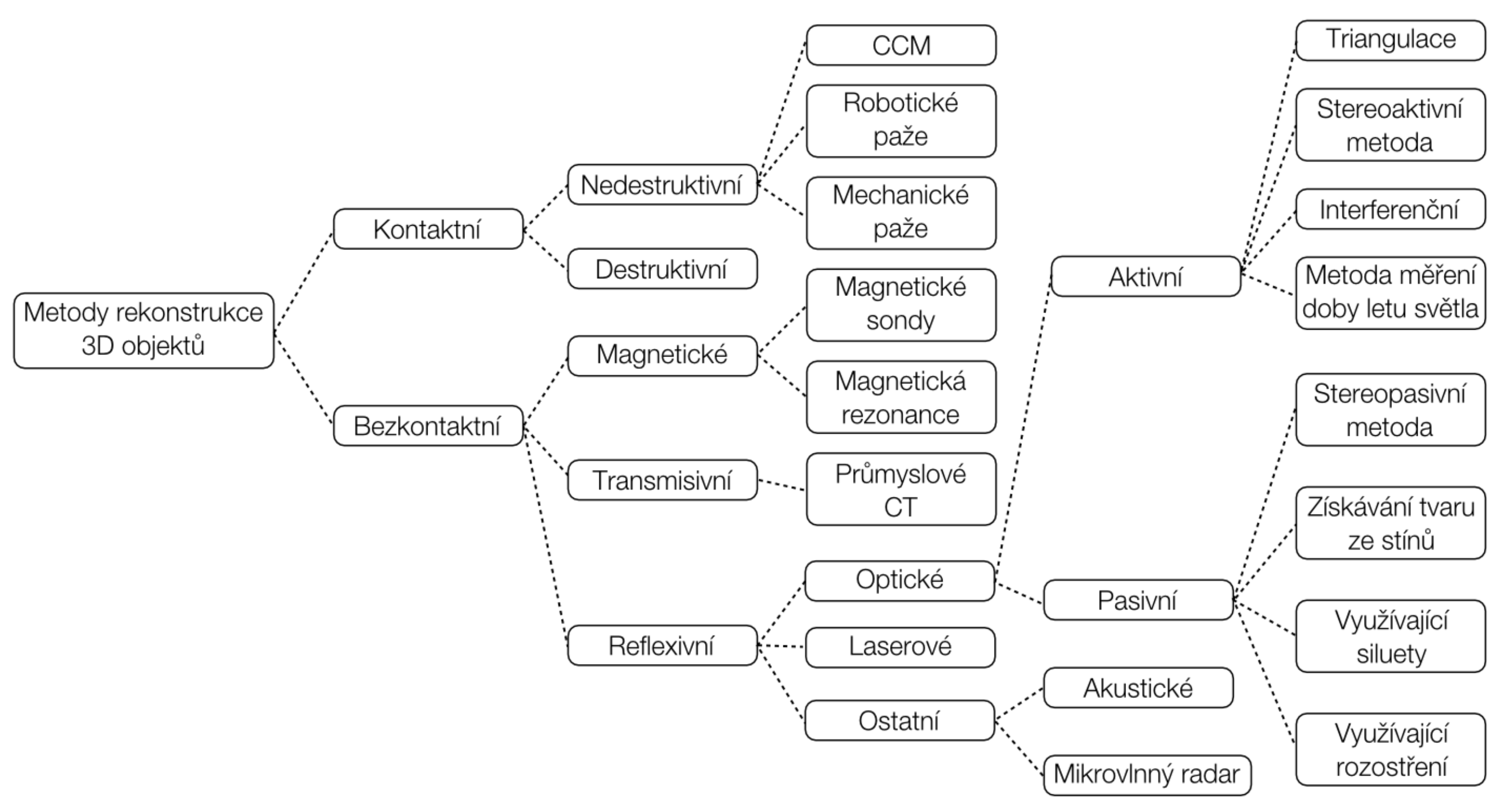
Classification of 3D scanners is possible in many ways. The selected classification takes as the main criterion contact and non-contact scanning methods. The most commonly used scanners are in the reflective branch. Laser methods can also fall under active optical methods using triangulation or the time-of-flight measurement method. In the taxonomy in the image, laser methods are separated out separately.
Contact
Contact occurs between the scanner and the scanned model.
Destructive
This type of scanner is somewhat atypical because it’s essentially a milling machine with a camera. At the beginning, the measured object needs to be cast into a block so that auxiliary material perfectly fills all cavities. The color of this material must be contrasting compared to the color of the scanned object. Such prepared part is mounted on the mill bed and thin layers of constant thickness are gradually milled off. Each newly revealed layer is always photographed and the image saved for later processing. The result is therefore a set of 2D photos with stored information about what Z height the photo was taken at. Software on each photo at the color transition of the cast object and auxiliary material extracts the boundary curve. This curve is represented as points in the plane. If curves from all milled levels are connected, then we get a 3D point cloud.
Non-destructive
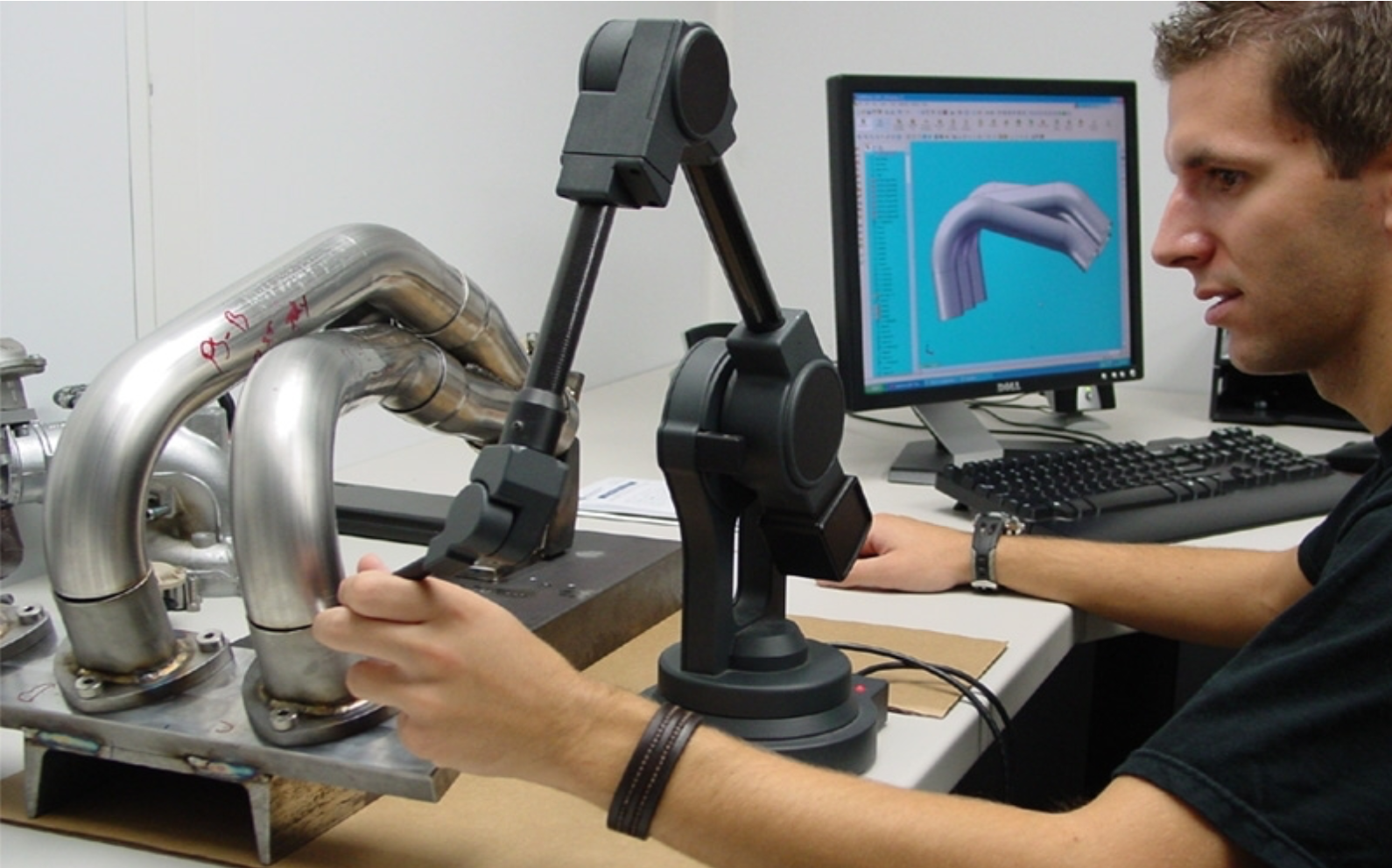
Non-destructive contact scanners include all, unlike destructive methods, the object is not damaged during digitization. Contact 3D scanners examine the object’s surface using physical tangible touch. While the object remains at rest attached to the base, a positioning arm on which a point or ball probe is mounted allows the user to pointwise capture 3D data from the physical object.
Non-contact
Magnetic Scanners
We can divide them into scanners with a magnetic probe or scanners using magnetic resonance. By using the second mentioned type of device, we can obtain information about the internal geometry of components. This is a non-destructive scanner working on the same principle as classical magnetic resonance used in healthcare. Devices are usually mobile and are used, for example, to check pipelines, boilers, or other closed vessels.
Transmissive Scanners
A representative of transmissive scanners are scanners using computed tomography (CT) technology. Just like scanners using magnetic resonance, this type of scanner can obtain data about the internal structure of the examined object. X-rays are used for information transfer. Unlike healthcare versions of CT, this use employs higher radiation intensity. These devices are still relatively rare, which is also proven by the fact that in the Czech Republic there is only one specimen.
Reflective Scanners
This category includes acoustic scanners (e.g., sonar), laser, but primarily optical. Optical scanners are the most widespread and most commonly used branch of 3D scanners. This results in the greatest number of various technological solutions and thus also further division.
Optical – Active 3D Scanners
Active optical methods are further divided according to what physical property of the given radiation is used for calculating the spatial coordinate of a point
Time of Flight
The simplest method is called "time of flight". This method is based on measuring the time it takes for the sent beam to return to the sensor after reflection from the object.
Triangulation
Another possibility is the "triangulation" method, which based on the known angle between projector and sensor, known distance of projector from sensor, and known position of the measured point on the sensor, can calculate the actual spatial point on the object’s surface.
Triangulation can be:
- active
- passive
Structured Light
Another active optical method is "structured light". This uses projection of a regular pattern onto the object and based on deformation of this pattern then calculates spatial coordinates of points. The advantage of this method is enormous speed at which the given object surface is scanned. It’s on the order of millions of points in a few seconds.
In practice, you can encounter this technology for example in
- Microsoft Kinect
- Assus Xtion
- Intel RealSense
- Mainly Time of flight
- used in industry
- Stereo active and passive
- active for example Ciclop/Horus
- Structured light
- Kinect
- RealSense
CloudCompare
CloudCompare is an open-source program for editing and modifying point clouds and 3D models. The program also allows calculating interesting data about similarities or measuring various distances and statistics.
In the field of 3D scanning, we’ll use it primarily for converting point clouds to triangular mesh.
Examples of Working with the Program
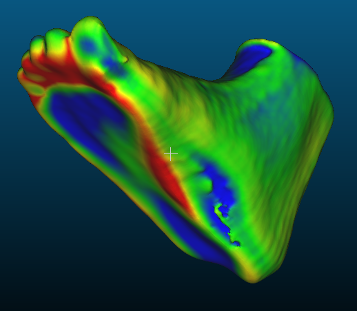
Reconstructing Foot Model
Required models are foot_scan.bin and foot_reference.stl. The foot model is from the portal Thingiverse, CC BY-NC 3.0 Voodoo Manufacturing.
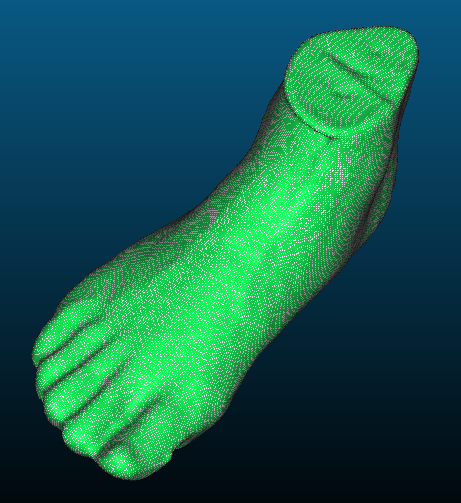
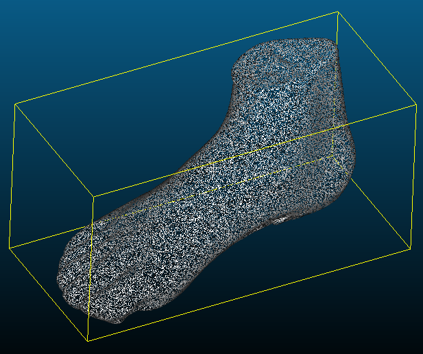
In the file foot_scan.bin there’s a point cloud created by scanning the foot model. Open it in the CloudCompare application.
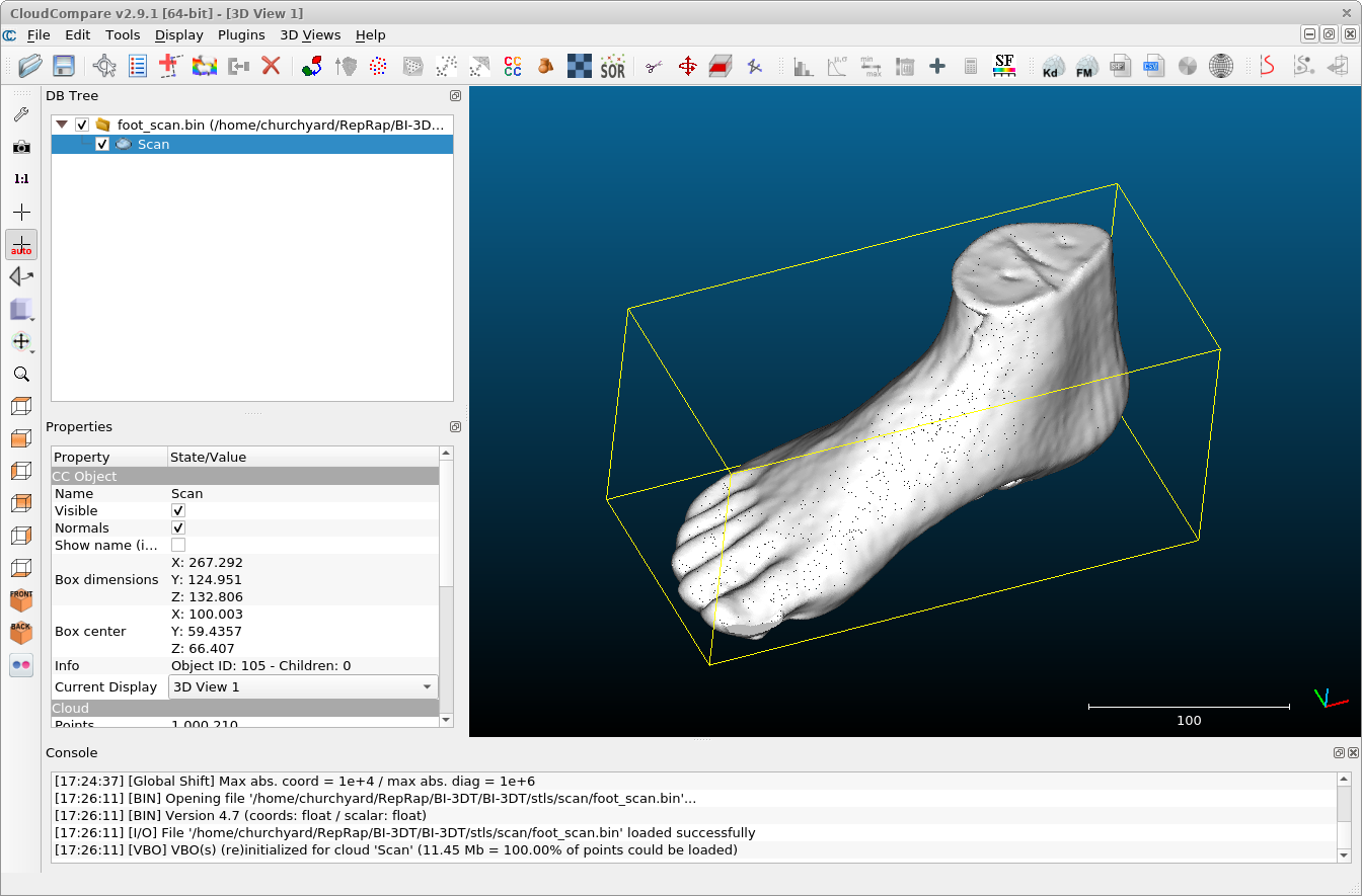
To work with the model, you need to select it in the upper left part of the program (DB Tree). The checkbox is for showing (or hiding) the model. The selected model is highlighted.
For reconstruction we’ll first use the entire cloud. For weaker computers this is not recommended; the cloud has about a million points and it could take a long time. Later we’ll show how to reconstruct a model from a smaller number of points.
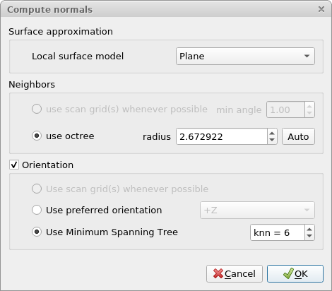
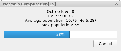
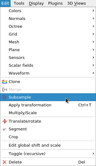
First you need to calculate normals using Edit → Normals → Compute. For our purposes, default values will suffice.
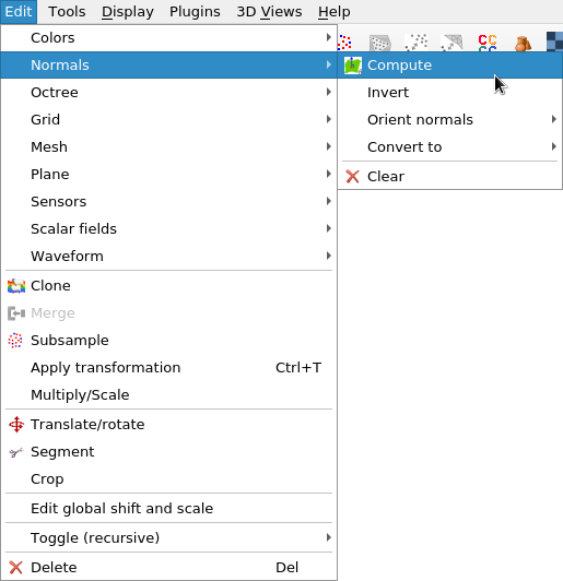
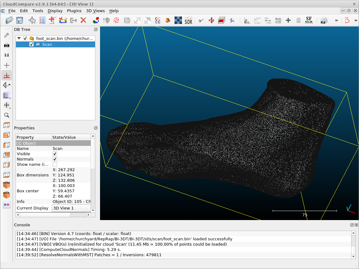
Sometimes normals are calculated reversed (they’re displayed in black). In such a case, they need to be inverted. If we didn’t do this, the reconstructed model would be turned inside out. Normals are inverted using Edit → Normals → Invert.

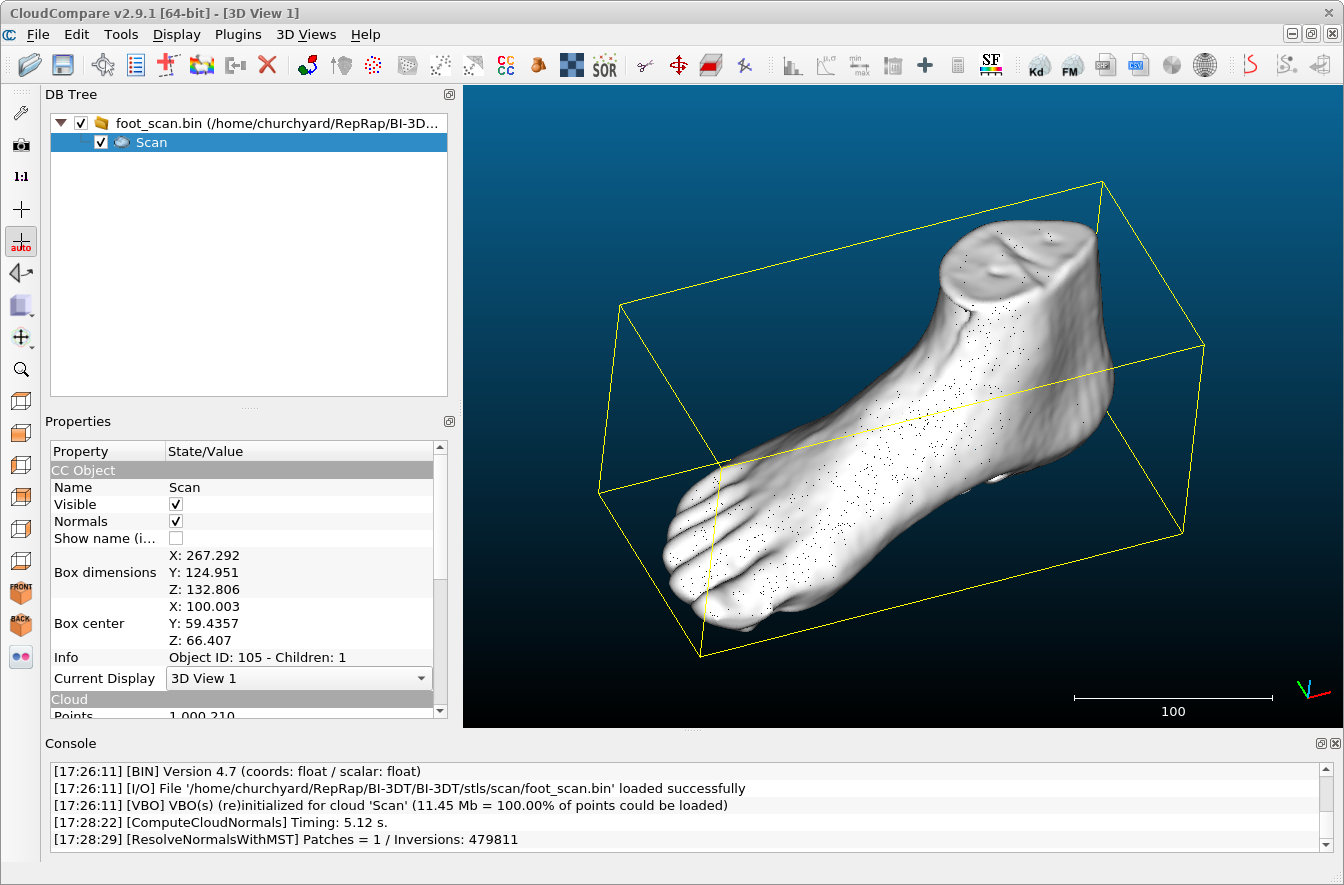
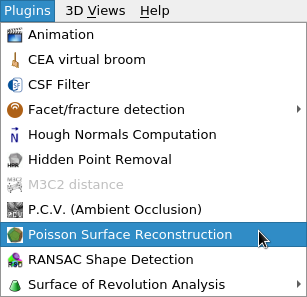
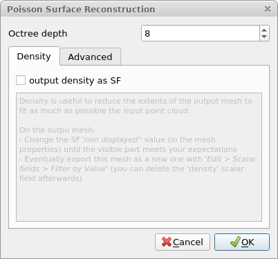
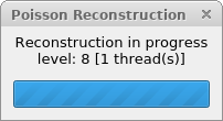
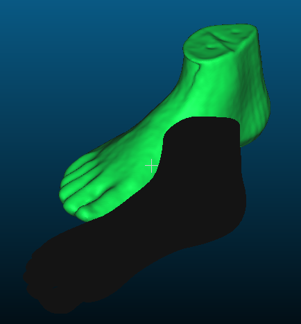
When we have normals, we can use Plugins → Poisson Surface Reconstruction.
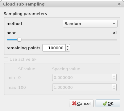
If the cloud is too large, we can subsample it before reconstruction: that is, get only part of the points. For our foot about a hundred thousand points suffice.
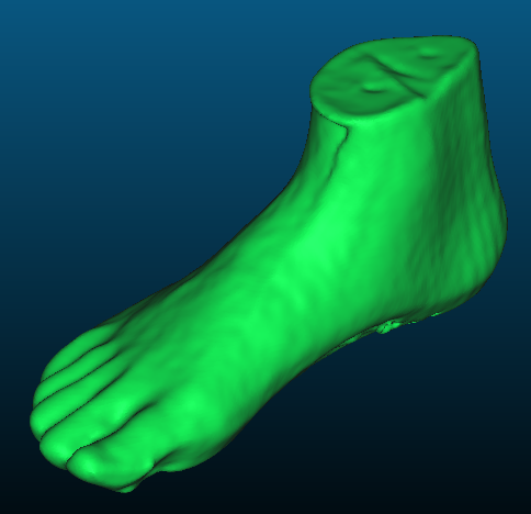
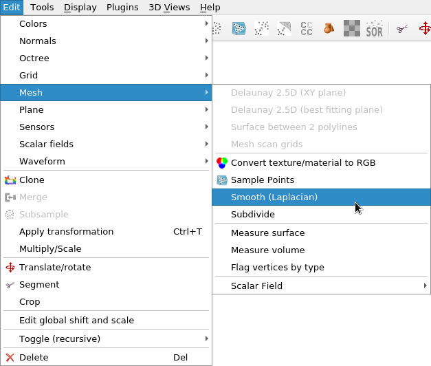
Sometimes it happens that the resulting mesh is too grainy. It’s possible to "to taste" smooth it using Edit → Mesh → Smooth (Laplacian).
You can also load a finished mesh into the program from the file foot_reference.stl (just open the file).
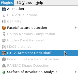
For clarity of mesh display you can use Plugins → P. C. V. (Ambient Occlusion).
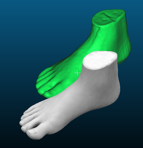
When we position the reconstructed and reference mesh at the same place, we can compare them. In the exercise we’ll show this; if you’re reading materials from home, you’ll learn more in the next example.
Garden Model: Registration of Two Scans
Required models are garden1.bin and garden2.bin, downloaded directly from the project CloudCompare, GPL 2+.
Brief sequence of steps (assumes watching video or attending exercise):
- Open both files.
- In Properties choose for both Colors → RGB.
- Using the Translate/rotate tool in the top bar, try to position the scans closer to each other.
- (optional) View Edit → Apply transformation.
- Select both files by clicking with Crtl key in DB Tree.
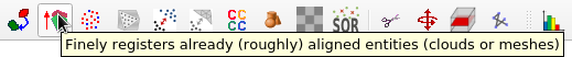
- From the toolbar select the Register enitites button (in newer version Finely register already (roughly) aligned entities (cloud or meshes)).
- Set Error difference or EMS difference to
1e-20. - Set Random sampling limit to
60000. - OK.
- In Properties again choose for both Colors → RGB.
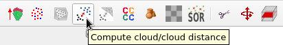
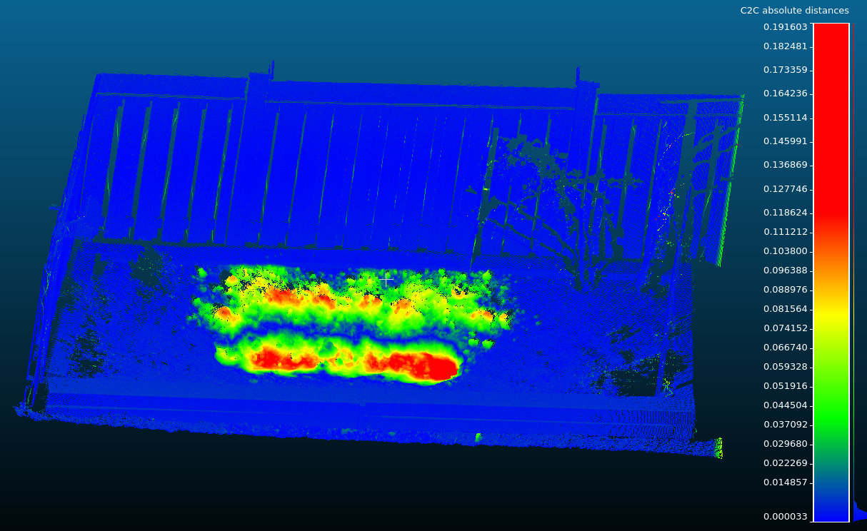
- From the toolbar select the Compute cloud/cloud distance button.
- Set model 1 as reference, Compute, OK.
- Display and select only the second model.
- In Properties check Colors → Scalar field, contains calculated distances.
- Properties → Color Scale → Visible.
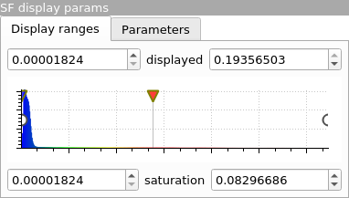
- SF display params: move sliders until result is "best".
Garden Model: Segmentation, Alignment by Reference Points
Required models are the same as above: garden1.bin and garden2.bin.
First we need two scans that are not so similar as above. To demonstrate this, we’ll cut out only the part with soil using the Segment tool.
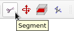
The tool is controlled with left mouse button; for confirmation use right button. Then select the cut-out polygon symbol and confirm with checkmark. The operation creates two new clouds in the tree.

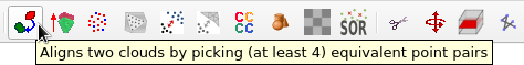
Then you need to use the tool Align two clouds by picking (at least 4) equivalents point pairs.
Then you can continue as in the previous example.
Useful Links
Guide to reconstructing a model using MeshLab or CloudCompare: Horus_Guide_to_post-processing_of_the_point_cloud.pdf